Computing α-diversity – Visualizing biodiversity data

Diversity indices are a common descriptive statistic used in biodiversity informatics. Diversity indices typically express the species richness of a given habitat or area. The α-diversity index is suitable when studying a single habitat and is expressed by a single number. There are several commonly used equations used to compute α-diversity. In this example, I will be using the Simpson’s diversity index, which is computed by the formula:

$D = 1 - \sum_{i=1}^{S}p_i^2$

Where S is the number of species in the sample and p is the proportion of a particular species. The Simpson’s diversity index is thus more influenced by common species rather than by rare species and is often considered to be an index reflecting the actual species diversity in a sample.

To illustrate this, I will use will use data obtained from GBIF. Remember, α-diversity is suitable for expressing the diversity within a single habitat, so I will obtain data accordingly. Here I chose the Tiergarten, a large (210 hectare) park in central Berlin.

Obtaining the data

In a previous post, I showed several methods to get data from GBIF. Here, I used the GBIF website to download a tab-separated list of occurrences in the chosen area. The area was selected using the location/polygon tool. I limited the results to birds (“Animalia/Chordata/Aves”) using the scientific name filter [1].

Cleaning the data

I opened the dataset using OpenRefine, which is a great tool for cleaning up data. The raw dataset lists 13552 observations.

I’ll be using species data for this example, so I dropped observations where the species is not specified (e.g. at genus level), using OpenRefine’s facet tool.
I also checked the license of each observation, and found that all observations in this particular dataset are under Creative commons licenses.
Diversity indices take the number of individuals into account, so I dropped observations where the individual count is not specified.
The year column shows that a couple of observations are historical, i.e. from the 19th century onwards. I dropped observations older than 10 years. While this 10 year limit is arbitrary, it allows to focus on the current biodiversity, rather than on the availabity of data in digital form.

I then exported the cleaned-up dataset as comma-separated-values (CSV). The final dataset has 8934 observations.

Counting the number of species in the dataset

I setup a Jupyter Notebook to do the calculations, using Python and pandas. You can see the calculations there. The dataset lists 126 species. The 10 most common species are:

species
Passer domesticus      6917
Corvus cornix          5284
Turdus merula          4178
Anas platyrhynchos     3873
Columba palumbus       3540
Grus grus              3165
Parus major            3091
Cyanistes caeruleus    2996
Columba livia          1827
Sturnus vulgaris       1804

That looks pretty reasonable, however cranes are most probably fly-overs.

Counting species vs. species diversity

So what’s wrong with just counting species and observations as a measure for biodiversity? Looking at the number of species by year illustrates the problem:

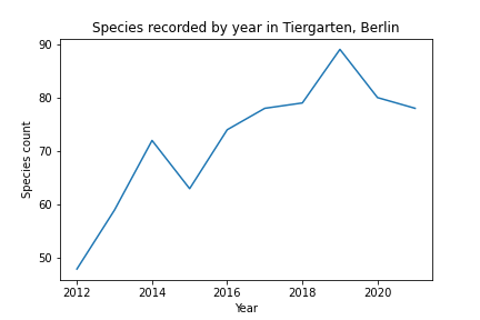
Does this mean that the number of species in Tiergarten has increased from 50 to 80 during the past 10 years? Certainly not. The graph just shows that as more data becomes available, rare species have a greater probability of being recorded.

Therefore, simply counting species is not a valid index of biodiversity.

The graph also shows that the number of species recorded has plateaud, i.e. the number of observations is so large, that all species in the area have been recorded.

Computing the diversity index

The Simpson’s diversity index is computed using the equation above. The calculations are in this Jupyter notebook. For the Tiergarten area, the result is

D = 0.9456

Interpretation

So what does this mean?

To interpret this result, one has to convert it to the corresponding “effective number of species”, i.e. the number of equally common species that would yield the same diversity index. For the Simpson’s diversity index, the effective number of species is given by [3]

$Dx = \frac{1}{1-D}$

where D is the Simpson’s diversity index. The effective number of species for Tiergarten is:

$Dx = \frac{1}{1-0.9456} \approx 18 [species]$

Having calculated a common diversity index for a specific area, based on GBIF data, and having computed the effective number of species, this last result could be used to compare the diversity between different areas on a linear scale, as well as to calculate a meaningful diversity fraction.

So let’s do this to compare the diversity in 2 different parks in Berlin. The calculations are in this Jupyter notebook.

Park	Species count	Diversity index	Effective species
Tiergarten [1]	126	0.95	18
Tempelhofer Feld [4]	241	0.91	11

So, while many more species have been recorded in Tempelhofer Feld, the effective species diversity in Tiergarten is close to 60% higher.

References

GBIF.org (12 March 2022) GBIF Occurrence Download https://doi.org/10.15468/dl.x3wym4
Jost, L. (2013). Measuring the diversity of a single community.
Jost, L. (2013) Effective number of species table
GBIF.org (14 March 2022) GBIF Occurrence Download https://doi.org/10.15468/dl.j6sv7h