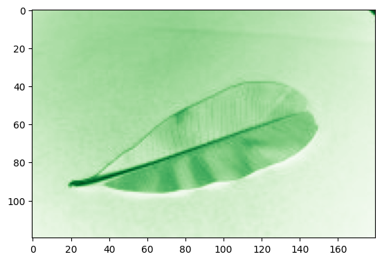
Plant leaf classification

There are important potential applications for a machine learning system than can classify plants. For example, current research on crop protection is using machine learning for precision weed and plant disease detection. The importance of moving away from traditional pesticide-based crop protection methods cannot be overstated, as demonstrated by the alarming rate at which flowering plants are evolving away from insect pollination.

I obtained a dataset of plant leaf images (Hussain, 2023) and compared three machine learning algorithms for classification: multilayer perceptron, random forest and support vector machine. The classifiers’ accuracy vary between 74% and 84% .

The Jupyter notebook with the full Python code can be accessed on Kaggle.
Storing a taxonomic tree in a relational database

Taxonomic trees are ubiquitous in biodiversity software. A very common application is using a tree to allow the users to browse the data. Other applications are: training classification models, curating a collection, visualizing research results etc.

Data is often stored in a relational database, such as MySQL. Unfortunately, relational databases are not particularly well suited for storing tree structures. Yet the choice of a database may be guided by more important requirements, and so the taxonomic tree is sometimes implemented as an afterthought. The result can be a structure that is difficult to maintain and to query, sometimes requiring more work than expected to maintain and finally yielding a less satisfying experience for the end user.

I will show some counterexamples, and how get a better result by using a data structure called “nested set”.

Continue reading “Storing a taxonomic tree in a relational database”

Computing α-diversity

Diversity indices are a common descriptive statistic used in biodiversity informatics. Diversity indices typically express the species richness of a given habitat or area. The α-diversity index is suitable when studying a single habitat and is expressed by a single number. There are several commonly used equations used to compute α-diversity. In this example, I will be using the Simpson’s diversity index, which is computed by the formula:

    \[D = 1 - \sum_{i=1}^{S}p_i^2\]

Where S is the number of species in the sample and p is the proportion of a particular species. The Simpson’s diversity index is thus more influenced by common species rather than by rare species and is often considered to be an index reflecting the actual species diversity in a sample.

To illustrate this, I will use will use data obtained from GBIF. Remember, α-diversity is suitable for expressing the diversity within a single habitat, so I will obtain data accordingly. Here I chose the Tiergarten, a large (210 hectare) park in central Berlin.

Continue reading “Computing α-diversity”

Using neural networks to classify 3D scans

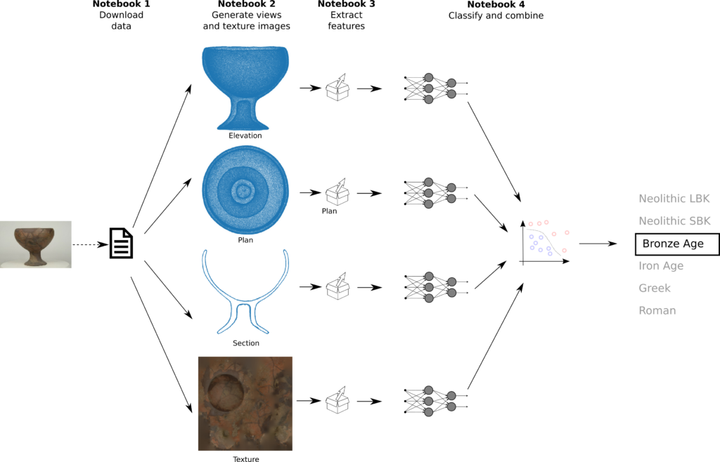
For my capstone project in machine learning at EPFL, I wrote a classifier capable of sorting 3D scans of archaeological objects by culture.

Digitization of museum collections is currently a major challenge faced by cultural heritage and natural history museums. Museums are expected to digitize the collections to improve not only the documentation of artifacts, but also their availability for research, reconstruction and outreach activities, and to make these digital representations available online.

Machine learning setup

Continue reading “Using neural networks to classify 3D scans”

Summarizing a text using topic modeling

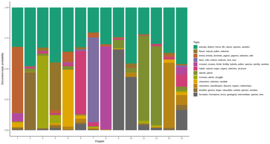
Much of biodiversity is discovered in museum collections, sometimes years after the specimen has been collected. Ploughing through expedition notes and logs is then required and therefore having a way to summarize the contents of a large text corpus can be very interesting. In this example, I will graphically summarize “On the Origin of Species” by Charles Darwin (it seemed a suitable choice) to demonstrate this technique.

Continue reading “Summarizing a text using topic modeling”

Comparing the distribution of Corvus corone and Corvus cornix

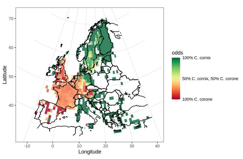
In this post, I will use a divergent color scale to plot two distributions on the same map. As an example, I chose to plot the European distribution of two species of corvids: the carrion crow (Corvus corone) and the hooded crow (Corvus cornix). There has been some adjustments to the taxonomical status of the hooded crow (see Parkin et al., 2003 for details), hoewever, currently, they are regarded as different species.

In this map, I will use a divergent color scale to show areas in Europe where each species is dominant, and also show areas where both species are present.

Distribution of Corvus corone and C. cornix in Europe
Continue reading “Comparing the distribution of Corvus corone and Corvus cornix

Simple distribution maps using ggplot

In a previous post, I discussed how to plot GBIF occurrence data using OpenStreetMaps. Here, I will plot a distribution map. Distribution maps differ from occurrence maps in that occurrences are aggregated and plotted as a heat map. Additionally, the map has to be projected using an equal area projection.
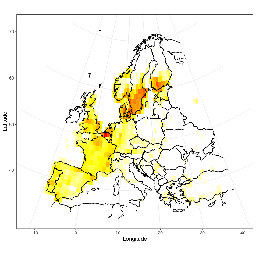
I will illustrate these two features by plotting the distribution of the tawny owl (Strix aluco) in Europe.

Distribution of the tawny owl in Europe
Continue reading “Simple distribution maps using ggplot”